From Surf Wiki (app.surf) — the open knowledge base
Tetration
Arithmetic operation
Arithmetic operation

In mathematics, tetration (or hyper-4) is an operation based on iterated, or repeated, exponentiation. There is no universal notation for tetration, though Knuth's up arrow notation \uparrow \uparrow and the left-exponent {}^{x}b are common.
Under the definition as repeated exponentiation, {^{n}a} means {a^{a^{\cdot^{\cdot^{a}}}}}, where n copies of a are iterated via exponentiation, right-to-left, i.e. the application of exponentiation n-1 times. The number n is called the height of the function, while a is called the base, analogous to exponentiation. It would be read as "the nth tetration of a". For example, 2 tetrated to 4 (or the fourth tetration of 2) is {^{4}2}=2^{2^{2^{2}}}=2^{2^{4}}=2^{16}=65536.
Tetration is the next hyperoperation after exponentiation, but before pentation. Along with the other hyperoperations, tetration is used for the notation of very large numbers. The name was coined by Reuben Goodstein from the prefix tetra- (meaning "four") and the word "iteration".
Tetration can also be defined recursively as : {a \uparrow \uparrow n} := \begin{cases} 1 &\text{if }n=0, \ a^{a \uparrow\uparrow (n-1)} &\text{if }n0. \end{cases} This form allows for the extension of tetration to more general domains than the natural numbers such as real, complex, or ordinal numbers.
The two inverses of tetration are called super-root and super-logarithm. They are respectively analogous to the operations of taking nth roots and taking logarithms. None of the three functions are elementary.
Introduction
The first four hyperoperations are shown here, with tetration being considered the fourth in the series. The unary operation succession, defined as a' = a + 1, is considered to be the zeroth operation.
- Addition a + n = a + \underbrace{1 + 1 + \cdots + 1}_n n copies of 1 added to a combined by succession.
- Multiplication a \times n = \underbrace{a + a + \cdots + a}_n n copies of a combined by addition.
- Exponentiation a^n = \underbrace{a \times a \times \cdots \times a}_n n copies of a combined by multiplication.
- Tetration {^{n}a} = \underbrace{a^{a^{\cdot^{\cdot^{a}}}}}_n n copies of a combined by exponentiation, right-to-left.
Importantly, nested exponents are interpreted from the top down: means and not
Succession, a_{n+1} = a_n + 1, is the most basic operation; while addition (a + n) is a primary operation, for addition of natural numbers it can be thought of as a chained succession of n successors of a; multiplication (a \times n) is also a primary operation, though for natural numbers it can analogously be thought of as a chained addition involving n numbers of a. Exponentiation can be thought of as a chained multiplication involving n numbers of a and tetration (^{n}a) as a chained power involving n numbers a. Each of the operations above are defined by iterating the previous one; however, unlike the operations before it, tetration is not an elementary function.
The parameter a is referred to as the base, while the parameter n may be referred to as the height. In the original definition of tetration, the height parameter must be a natural number; for instance, it would be illogical to say "three raised to itself negative five times" or "four raised to itself one half of a time." However, just as addition, multiplication, and exponentiation can be defined in ways that allow for extensions to real and complex numbers, several attempts have been made to generalize tetration to negative numbers, real numbers, and complex numbers. One such way for doing so is using a recursive definition for tetration; for any positive real a 0 and non-negative integer n \ge 0, we can define ,! {^{n}a} recursively as: : {^{n}a} := \begin{cases} 1 &\text{if }n=0 \ a^{\left(^{(n-1)}a\right)} &\text{if }n0 \end{cases} The recursive definition is equivalent to repeated exponentiation for natural heights; however, this definition allows for extensions to the other heights such as ^{0}a, ^{-1}a, and ^{i}a as well – many of these extensions are areas of active research.
Terminology
There are many terms for tetration, each of which has some logic behind it, but some have not become commonly used for one reason or another. Here is a comparison of each term with its rationale and counter-rationale.
- The term tetration, introduced by Goodstein in his 1947 paper Transfinite Ordinals in Recursive Number Theory (generalizing the recursive base-representation used in Goodstein's theorem to use higher operations), has gained dominance. It was also popularized in Rudy Rucker's Infinity and the Mind.
- The term superexponentiation was published by Bromer in his paper Superexponentiation in 1987. It was used earlier by Ed Nelson in his book Predicative Arithmetic, Princeton University Press, 1986.
- The term hyperpower is a natural combination of hyper and power, which aptly describes tetration. The problem lies in the meaning of hyper with respect to the hyperoperation sequence. When considering hyperoperations, the term hyper refers to all ranks, and the term super refers to rank 4, or tetration. So under these considerations hyperpower is misleading, since it is only referring to tetration.
- The term power tower is occasionally used, in the form "the power tower of order n" for {\ \atop {\ }} }}}} \atop n}. Exponentiation is easily misconstrued: note that the operation of raising to a power is right-associative (see below). Tetration is iterated exponentiation (call this right-associative operation ^), starting from the top right side of the expression with an instance a^a (call this value c). Exponentiating the next leftward a (call this the 'next base' b), is to work leftward after obtaining the new value b^c. Working to the left, use the next a to the left, as the base b, and evaluate the new b^c. 'Descend down the tower' in turn, with the new value for c on the next downward step.
Owing in part to some shared terminology and similar notational symbolism, tetration is often confused with closely related functions and expressions. Here are a few related terms:
| Terminology | Form | Tetration | Iterated exponentials | Nested exponentials (also towers) | Infinite exponentials (also towers) |
|---|---|---|---|---|---|
| a^{a^{\cdot^{\cdot^{a^a}}}} | |||||
| a^{a^{\cdot^{\cdot^{a^x}}}} | |||||
| a_1^{a_2^{\cdot^{\cdot^{a_n}}}} | |||||
| a_1^{a_2^{a_3^{\cdot^{\cdot^\cdot}}}} |
In the first two expressions a is the base, and the number of times a appears is the height (add one for x). In the third expression, n is the height, but each of the bases is different.
Care must be taken when referring to iterated exponentials, as it is common to call expressions of this form iterated exponentiation, which is ambiguous, as this can either mean iterated powers or iterated exponentials.
Notation
There are many different notation styles that can be used to express tetration. Some notations can also be used to describe other hyperoperations, while some are limited to tetration and have no immediate extension.
| Name | Form | Description | Knuth's up-arrow notation | Conway chained arrow notation | Ackermann function | Iterated exponential notation | Hooshmand notations | Hyperoperation notations | Double caret notation |
|---|---|---|---|---|---|---|---|---|---|
| \begin{align} | Allows extension by putting more arrows, or, even more powerfully, an indexed arrow. | ||||||||
| a \rightarrow n \rightarrow 2 | Allows extension by increasing the number 2 (equivalent with the extensions above), but also, even more powerfully, by extending the chain. | ||||||||
| {}^{n}2 = \operatorname{A}(4, n - 3) + 3 | Allows the special case a=2 to be written in terms of the Ackermann function. | ||||||||
| \exp_a^n(1) | Allows simple extension to iterated exponentials from initial values other than 1. | ||||||||
| \begin{align} | Used by M. H. Hooshmand [2006]. | ||||||||
| \begin{align} | Allows extension by increasing the number 4; this gives the family of hyperoperations. | ||||||||
| Since the up-arrow is used identically to the caret (`^`), tetration may be written as (`^^`); convenient for ASCII. |
One notation above uses iterated exponential notation; this is defined in general as follows:
: \exp_a^n(x) = a^{a^{\cdot^{\cdot^{a^x}}}} with n as.
There are not as many notations for iterated exponentials, but here are a few:
| Name | Form | Description | Standard notation | Knuth's up-arrow notation | Text notation | J notation | Infinity barrier notation | |
|---|---|---|---|---|---|---|---|---|
| \exp_a^n(x) | Euler coined the notation \exp_a(x) = a^x, and iteration notation f^n(x) has been around about as long. | |||||||
| (a{\uparrow}^2(x)) | Allows for super-powers and super-exponential function by increasing the number of arrows; used in the article on large numbers. | |||||||
| Based on standard notation; convenient for ASCII. | ||||||||
| Repeats the exponentiation. See J (programming language). | ||||||||
| a\uparrow\uparrow n | x | Jonathan Bowers coined this, and it can be extended to higher hyper-operations. |
Examples
Because of the extremely fast growth of tetration, most values in the following table are too large to write in scientific notation. In these cases, iterated exponential notation is used to express them in base 10. The values containing a decimal point are approximate. Usually, the limit that can be calculated in a numerical calculation program such as Wolfram Alpha is 3↑↑4, and the number of digits up to 3↑↑5 can be expressed.
| x | {}^{2}x | {}^{3}x | {}^{4}x | {}^{5}x | {}^{6}x | {}^{7}x | 1 | 2 | 3 | 4 | 5 | 6 | 7 | 8 | 9 | 10 |
|---|---|---|---|---|---|---|---|---|---|---|---|---|---|---|---|---|
| 1 | 1 | 1 | 1 | 1 | 1 | |||||||||||
| 4 (2) | 16 (2) | 65,536 (2) | 2.00353 × 10 (2) | \exp_{10}^3(4.29508) (10) | \exp_{10}^4(4.29508) | |||||||||||
| 27 (3) | 7,625,597,484,987 | 1.25801 × 10 (3) | \exp_{10}^4(1.09902) | \exp_{10}^5(1.09902) | \exp_{10}^6(1.09902) | |||||||||||
| 256 (4) | 1.34078 × 10 (4) | \exp_{10}^3(2.18726) (2.3610×10) | \exp_{10}^4(2.18726) | \exp_{10}^5(2.18726) | \exp_{10}^6(2.18726) | |||||||||||
| 3,125 (5) | 1.91101 × 10 (5) | \exp_{10}^3(3.33928) (10) | \exp_{10}^4(3.33928) | \exp_{10}^5(3.33928) | \exp_{10}^6(3.33928) | |||||||||||
| 46,656 (6) | 2.65912 × 10 (6) | \exp_{10}^3(4.55997) (10) | \exp_{10}^4(4.55997) | \exp_{10}^5(4.55997) | \exp_{10}^6(4.55997) | |||||||||||
| 823,543 (7) | 3.75982 × 10 (7823,543) | \exp_{10}^3(5.84259) (3.17742 × 10 digits) | \exp_{10}^4(5.84259) | \exp_{10}^5(5.84259) | \exp_{10}^6(5.84259) | |||||||||||
| 16,777,216 (8) | 6.01452 × 10 | \exp_{10}^3(7.18045) (5.43165 × 10 digits) | \exp_{10}^4(7.18045) | \exp_{10}^5(7.18045) | \exp_{10}^6(7.18045) | |||||||||||
| 387,420,489 (9) | 4.28125 × 10 | \exp_{10}^3(8.56784) (4.08535 × 10 digits) | \exp_{10}^4(8.56784) | \exp_{10}^5(8.56784) | \exp_{10}^6(8.56784) | |||||||||||
| 10,000,000,000 (10) | 10 | \exp_{10}^4(1) (10 + 1 digits) | \exp_{10}^5(1) | \exp_{10}^6(1) | \exp_{10}^7(1) |
Remark: If x does not differ from 10 by orders of magnitude, then for all k \ge3,~ ^mx =\exp_{10}^k z,~z1 \Rightarrow^{m+1}x = \exp_{10}^{k+1} z' \text{ with }z' \approx z. For example, z - z' in the above table, and the difference is even smaller for the following rows.
Extensions
Tetration can be extended in two different ways; in the equation ^na!, both the base a and the height n can be generalized using the definition and properties of tetration. Although the base and the height can be extended beyond the non-negative integers to different domains, including {^n 0}, complex functions such as {}^{n}i, and heights of infinite n, the more limited properties of tetration reduce the ability to extend tetration.
Extension of domain for bases
Base zero
The exponential 0^0 is not consistently defined. Thus, the tetrations ,{^{n}0} are not clearly defined by the formula given earlier. However, \lim_{x\rightarrow0} {}^{n}x is well defined, and exists: :\lim_{x\rightarrow0} {}^{n}x = \begin{cases} 1, & n \text{ even} \ 0, & n \text{ odd} \end{cases}
Thus we could consistently define {}^{n}0 = \lim_{x\rightarrow 0} {}^{n}x. This is analogous to defining 0^0 = 1.
Under this extension, {}^{0}0 = 1, so the rule {^{0}a} = 1 from the original definition still holds.
Complex bases


Since complex numbers can be raised to powers, tetration can be applied to bases of the form (where a and b are real). For example, in z with , tetration is achieved by using the principal branch of the natural logarithm; using Euler's formula we get the relation:
: i^{a+bi} = e^{\frac{1}{2}{\pi i} (a + bi)} = e^{-\frac{1}{2}{\pi b}} \left(\cos{\frac{\pi a}{2}} + i \sin{\frac{\pi a}{2}}\right)
This suggests a recursive definition for given any : : \begin{align} a' &= e^{-\frac{1}{2}{\pi b}} \cos{\frac{\pi a}{2}} \[2pt] b' &= e^{-\frac{1}{2}{\pi b}} \sin{\frac{\pi a}{2}} \end{align}
The following approximate values can be derived:
| {}^{n}i | Approximate value | {}^{1}i = i | {}^{2}i = i^{\left({}^{1}i\right)} | {}^{3}i = i^{\left({}^{2}i\right)} | {}^{4}i = i^{\left({}^{3}i\right)} | {}^{5}i = i^{\left({}^{4}i\right)} | {}^{6}i = i^{\left({}^{5}i\right)} | {}^{7}i = i^{\left({}^{6}i\right)} | {}^{8}i = i^{\left({}^{7}i\right)} | {}^{9}i = i^{\left({}^{8}i\right)} |
|---|---|---|---|---|---|---|---|---|---|---|
| *i* | ||||||||||
| 0.2079 | ||||||||||
| 0.9472 + 0.3208*i* | ||||||||||
| 0.0501 + 0.6021*i* | ||||||||||
| 0.3872 + 0.0305*i* | ||||||||||
| 0.7823 + 0.5446*i* | ||||||||||
| 0.1426 + 0.4005*i* | ||||||||||
| 0.5198 + 0.1184*i* | ||||||||||
| 0.5686 + 0.6051*i* |
Solving the inverse relation, as in the previous section, yields the expected and , with negative values of n giving infinite results on the imaginary axis. Plotted in the complex plane, the entire sequence spirals to the limit 0.4383 + 0.3606i, which could be interpreted as the value where n is infinite.
Such tetration sequences have been studied since the time of Euler, but are poorly understood due to their chaotic behavior. Most published research historically has focused on the convergence of the infinitely iterated exponential function. Current research has greatly benefited by the advent of powerful computers with fractal and symbolic mathematics software. Much of what is known about tetration comes from general knowledge of complex dynamics and specific research of the exponential map.
Extensions of the domain for different heights
Infinite heights


Tetration can be extended to infinite heights; i.e., for certain a and n values in {}^{n}a, there exists a well defined result for an infinite n. This is because for bases within a certain interval, tetration converges to a finite value as the height tends to infinity. For example, \sqrt{2}^{\sqrt{2}^{\sqrt{2}^{\cdot^{\cdot^{\cdot}}}}} converges to 2, and can therefore be said to be equal to 2. The trend towards 2 can be seen by evaluating a small finite tower:
: \begin{align} \sqrt{2}^{\sqrt{2}^{\sqrt{2}^{\sqrt{2}^{\sqrt{2}^{1.414}}}}} &\approx \sqrt{2}^{\sqrt{2}^{\sqrt{2}^{\sqrt{2}^{1.63}}}} \ &\approx \sqrt{2}^{\sqrt{2}^{\sqrt{2}^{1.76}}} \ &\approx \sqrt{2}^{\sqrt{2}^{1.84}} \ &\approx \sqrt{2}^{1.89} \ &\approx 1.93 \end{align}
In general, the infinitely iterated exponential x^{x^{\cdot^{\cdot^{\cdot}}}}!!, defined as the limit of {}^{n}x as n goes to infinity, converges for e ≤ x ≤ e, roughly the interval from 0.066 to 1.44, a result shown by Leonhard Euler. The limit, should it exist, is a positive real solution of the equation . Thus, . The limit defining the infinite exponential of x does not exist when x e because the maximum of y is e. The limit also fails to exist when {{math|0
This may be extended to complex numbers z with the definition: : {}^{\infty}z = z^{z^{\cdot^{\cdot^{\cdot}}}} = e^{-\mathrm{W}(-\ln{z})} = \frac{\mathrm{W}(-\ln{z})}{-\ln{z}} ~, where W represents Lambert's W function. This formula follows from the assumption that z^{z^{\cdot^{\cdot^{\cdot}}}} = a converges, and thus z^a = a, z = a^{1/a}, 1/z = (1/a)^{1/a} = {}^2(1/a), and 1/a = \mathrm{ssrt}(1/z) = e^{W(\ln(1/z))} (see square super-root below).
As the limit (if existent on the positive real line, i.e. for e ≤ x ≤ e) must satisfy we see that is (the lower branch of) the inverse function of .
Negative heights
We can reverse the recursive rule for tetration, : {^{k+1}a} = a^{\left({^{k}a}\right)},
to write: : ^{k}a = \log_a \left(^{k+1}a\right).
Substituting −1 for k gives : {}^{-1}a = \log_{a} \left({}^0 a\right) = \log_a 1 = 0.
Smaller negative values cannot be well defined in this way. Substituting −2 for k in the same equation gives : {}^{-2}a = \log_{a} \left( {}^{-1}a \right) = \log_a 0 = -\infty
which is not well defined. They can, however, sometimes be considered sets.
For n = 1, any definition of ,! {^{-1}1} is consistent with the rule because : {^{0}1} = 1 = 1^n for any ,! n = {^{-1}1}.
Linear approximation for real heights
A linear approximation (solution to the continuity requirement, approximation to the differentiability requirement) is given by: : {}^{x}a \approx \begin{cases} \log_a\left(^{x+1}a\right) & x \le -1 \ 1 + x & -1 a^{\left(^{x-1}a\right)} & 0 \end{cases}
hence:
| Approximation | Domain | {}^x a \approx x + 1 | {}^x a \approx a^x | {}^x a \approx a^{a^{(x-1)}} | |
|---|---|---|---|---|---|
| for {{math | −1 | ||||
| for {{math | 0 | ||||
| for {{math | 1 |
and so on. However, it is only piecewise differentiable; at integer values of x, the derivative is multiplied by \ln{a}. It is continuously differentiable for x -2 if and only if a = e. For example, using these methods {}^\frac{\pi}{2}e \approx 5.868... and {}^{-4.3}0.5 \approx 4.03335...
A main theorem in Hooshmand's paper states: Let 0 . If f:(-2, +\infty)\rightarrow \mathbb{R} is continuous and satisfies the conditions:
- f(x) = a^{f(x-1)} ;; \text{for all} ;; x -1, ; f(0) = 1,
- f is differentiable on ,
- f^\prime is a nondecreasing or nonincreasing function on ,
- f^\prime \left(0^+\right) = (\ln a) f^\prime \left(0^-\right) \text{ or } f^\prime \left(-1^+\right) = f^\prime \left(0^-\right).
then f is uniquely determined through the equation : f(x) = \exp^{[x]}_a \left(a^{(x)}\right) = \exp^{[x+1]}_a((x)) \quad \text{for all} ; ; x -2,
where (x) = x - [x] denotes the fractional part of x and \exp^{[x]}_a is the [x]-iterated function of the function \exp_a.
The proof is that the second through fourth conditions trivially imply that f is a linear function on .
The linear approximation to natural tetration function {}^xe is continuously differentiable, but its second derivative does not exist at integer values of its argument. Hooshmand derived another uniqueness theorem for it which states:
If f: (-2, +\infty)\rightarrow \mathbb{R} is a continuous function that satisfies:
- f(x) = e^{f(x-1)} ;; \text{for all} ;; x -1, ; f(0) = 1,
- f is convex on ,
- f^\prime \left(0^-\right) \leq f^\prime \left(0^+\right).
then f = \text{uxp}. [Here f = \text{uxp} is Hooshmand's name for the linear approximation to the natural tetration function.]
The proof is much the same as before; the recursion equation ensures that f^\prime (-1^+) = f^\prime (0^+), and then the convexity condition implies that f is linear on .
Therefore, the linear approximation to natural tetration is the only solution of the equation f(x) = e^{f(x-1)} ;; (x -1) and f(0) = 1 which is convex on . All other sufficiently-differentiable solutions must have an inflection point on the interval .
Higher order approximations for real heights

Beyond linear approximations, a quadratic approximation (to the differentiability requirement) is given by: : {}^{x}a \approx \begin{cases} \log_a\left({}^{x+1}a\right) & x \le -1 \ 1 + \frac{2\ln(a)}{1 ;+; \ln(a)}x - \frac{1 ;-; \ln(a)}{1 ;+; \ln(a)}x^2 & -1 a^{\left({}^{x-1}a\right)} & x 0 \end{cases}
which is differentiable for all x 0, but not twice differentiable. For example, {}^\frac{1}{2}2 \approx 1.45933... If a = e this is the same as the linear approximation.
Because of the way it is calculated, this function does not "cancel out", contrary to exponents, where \left(a^\frac{1}{n}\right)^n = a. Namely, : {}^n\left({}^\frac{1}{n} a\right) = \underbrace{ \left({}^\frac{1}{n}a\right)^{ \left({}^\frac{1}{n}a\right)^{ \cdot^{\cdot^{\cdot^{\cdot^{ \left({}^\frac{1}{n}a\right) } } }_n \neq a .
Just as there is a quadratic approximation, cubic approximations and methods for generalizing to approximations of degree n also exist, although they are much more unwieldy.
Complex heights

In 2017, it was proved{{cite journal |author-first1=W. |author-last1=Paulsen |author-first2=S. |author-last2=Cowgill F(z + 1) = \exp\bigl(F(z)\bigr) (equivalently F(z+1) = b^{F(z)} when b=e), with the auxiliary conditions F(0) = 1, and F(z) \to \xi_{\pm} (the attracting/repelling fixed points of the logarithm, roughly 0.318 \pm 1.337,\mathrm{i}) as z \to \pm i\infty. Moreover, F is holomorphic on all of \mathbb{C} except for the cut along the real axis at z \le -2. This construction was first conjectured by Kouznetsov (2009){{cite journal |author-first=D. |author-last=Kouznetsov |author-first=H. |author-last=Kneser |author-first=W. |author-last=Paulsen
In May 2025, Vey gave a unified, holomorphic extension for arbitrary complex bases b\in \mathbb{C}\setminus{0,1} and complex heights z\in\mathbb{C} by means of Schröder’s equation. In particular, one constructs a linearizing coordinate near the attracting (or repelling) fixed point of the map f(w)=b^w, and then patches together two analytic expansions (one around each fixed point) to produce a single function F_{b}(z) that satisfies F_{b}(z+1)=b^{,F_{b}(z)} and F_{b}(0)=1 on all of \mathbb{C}. The key step is to define \displaystyle \Phi_{b}(w)=\lim_{n\to\infty};s^{n}\Bigl(f^{\circ n}(w)-\alpha\Bigr), where \alpha is a fixed point of f(w)=b^w, s = f'(\alpha), and f^{\circ n} denotes n-fold iteration. One then solves Schröder’s functional equation \Phi_{b}\bigl(b^{,w}\bigr);=;s;\Phi_{b}(w) locally (for w near \alpha), extends both branches holomorphically, and glues them so that there is no monodromy except the known cut-lines. Vey also provides explicit series for the coefficients a_{n}^{(b)} in the local Schröder expansion: \Phi_{b}(w) = \sum_{n=0}^{\infty} a_{n}^{(b)},(w-\alpha)^{n}, and gives rigorous bounds proving factorial convergence of a_{n}^{(b)}.{{cite web |author-first=Vincent |author-last=Vey
Using Kneser’s (and Vey’s) tetration, example values include {}^{\tfrac{\pi}{2}}e \approx 5.82366\ldots, {}^{\tfrac{1}{2}}2 \approx 1.45878\ldots, and {}^{\tfrac{1}{2}}e \approx 1.64635\ldots.
The requirement that tetration be holomorphic on all of \mathbb{C} (except for the known cuts) is essential for uniqueness. If one relaxes holomorphicity, there are infinitely many real‐analytic “solutions” obtained by pre‐ or post‐composing with almost‐periodic perturbations. For example, for any fast‐decaying real sequences {\alpha_{n}} and {\beta_{n}}, one can set S(z)
F_{b}\Bigl(, z +\sum_{n=1}^{\infty}\sin(2\pi n,z),\alpha_{n} +\sum_{n=1}^{\infty}\bigl[1 - \cos(2\pi n,z)\bigr],\beta_{n} \Bigr), which still satisfies S(z+1)=b^{S(z)} and S(0)=1, but has additional singularities creeping in from the imaginary direction.
<!-- Example of “calling” Vey’s solution in pseudocode (series form) -->
function ComplexTetration(b, z):
    # 1) Find attracting fixed point alpha of w ↦ b^w
    α ← the unique solution of α = b^α near the real line
    # 2) Compute multiplier s = b^α · ln(b)
    s ← b**α * log(b)
    # 3) Solve Schröder’s equation coefficients {a_n} around α:
    #    Φ_b(w) = ∑_{n=0}^∞ a_n · (w − α)^n,   Φ_b(b^w) = s · Φ_b(w)
    {a_n} ← SolveLinearSystemSchroeder(b, α, s)
    # 4) Define inverse φ_b⁻¹ via the local power series around 0
    φ_inv(u) = α + ∑_{n=1}^∞ c_n · u^n   # (coefficients c_n from series inversion)
    # 5) Put F_b(z) = φ_b⁻¹(s^(-z) · Φ_b(1))
    return φ_inv( s^(−z) * ∑_{n=0}^∞ a_n · (1 − α)^n )
series converges for all w in a suitable neighborhood of α; see Vey 2025. --
Ordinal tetration
Tetration can be defined for ordinal numbers via transfinite induction. For all α and all β 0: {}^0\alpha = 1 {}^\beta\alpha = \sup({\alpha^{{}^\gamma\alpha} : \gamma
Non-elementary recursiveness
Tetration (restricted to \mathbb{N}^2) is not an elementary recursive function. One can prove by induction that for every elementary recursive function f, there is a constant c such that : f(x) \leq \underbrace{2^{2^{\cdot^{\cdot^{x}}}}}_c. We denote the right hand side by g(c, x). Suppose on the contrary that tetration is elementary recursive. g(x, x)+1 is also elementary recursive. By the above inequality, there is a constant c such that g(x,x) +1 \leq g(c, x). By letting x=c, we have that g(c,c) + 1 \leq g(c, c), a contradiction.
Inverse operations
Exponentiation has two inverse operations; roots and logarithms. Analogously, the inverses of tetration are often called the super-root, and the super-logarithm (In fact, all hyperoperations greater than or equal to 3 have analogous inverses); e.g., in the function {^3}y=x, the two inverses are the cube super-root of y and the super-logarithm base y of x.
Super-root
The super-root is the inverse operation of tetration with respect to the base: if ^n y = x, then y is an nth super-root of x (\sqrt[n]{x}_s or \sqrt[4]{x}_s).
For example, : ^4 2 = 2^{2^{2^{2}}} = 65{,}536
so 2 is the 4th super-root of 65,536 \left(\sqrt[4]{65{,}536}_s =2\right).
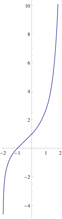
Square super-root
.svg)
The 2nd-order super-root, square super-root, or super square root has two equivalent notations, \mathrm{ssrt}(x) and \sqrt{x}_s. It is the inverse of ^2 x = x^x and can be represented with the Lambert W function:
: \mathrm{ssrt}(x)=\exp(W(\ln x))=\frac{\ln x}{W(\ln x)} or : \sqrt{x}_s=e^{W(\ln x)}
The function also illustrates the reflective nature of the root and logarithm functions as the equation below only holds true when y = \mathrm{ssrt}(x):
: \sqrt[y]{x} = \log_y x
Like square roots, the square super-root of x may not have a single solution. Unlike square roots, determining the number of square super-roots of x may be difficult. In general, if e^{-1/e}, then x has two positive square super-roots between 0 and 1 calculated using formulas:\sqrt{x}s=\left{e^{W{-1}(\ln x)};e^{W_{0}(\ln x)}\right}; and if x 1, then x has one positive square super-root greater than 1 calculated using formulas: \sqrt{x}s=e^{W{0}(\ln x)}. If x is positive and less than e^{-1/e} it does not have any real square super-roots, but the formula given above yields countably infinitely many complex ones for any finite x not equal to 1. The function has been used to determine the size of data clusters.
At x = 1 :
Other super-roots
One of the simpler and faster formulas for a third-degree super-root is the recursive formula. If y = x^{x^x} then one can use:
- x_0 = 1
- x_{n+1} = \exp(W(W(x_n\ln y))) This recursive formula makes use of the explicit representation of the square super-root via the Lambert W function given above, as we can represent y = x^{x^x} in the form of y^x = (x^x)^{(x^x)} and apply the square super-root twice: x = \mathrm{ssrt}(\mathrm{ssrt}(y^x)).
For each integer n 2, the function x is defined and increasing for x ≥ 1, and , so that the nth super-root of x, \sqrt[n]{x}_s, exists for x ≥ 1.
However, if the linear approximation above is used, then ^y x = y + 1 if {{math|−1 ^y \sqrt{y + 1}_s cannot exist.
In the same way as the square super-root, terminology for other super-roots can be based on the normal roots: "cube super-roots" can be expressed as \sqrt[3]{x}_s; the "4th super-root" can be expressed as \sqrt[4]{x}_s; and the "nth super-root" is \sqrt[n]{x}_s. Note that \sqrt[n]{x}_s may not be uniquely defined, because there may be more than one n root. For example, x has a single (real) super-root if n is odd, and up to two if n is even.
Just as with the extension of tetration to infinite heights, the super-root can be extended to , being well-defined if 1/e ≤ x ≤ e. Note that x = {^\infty y} = y^{\left[^\infty y\right]} = y^x, and thus that y = x^{1/x} . Therefore, when it is well defined, \sqrt[\infty]{x}_s = x^{1/x} and, unlike normal tetration, is an elementary function. For example, \sqrt[\infty]{2}_s = 2^{1/2} = \sqrt{2}.
It follows from the Gelfond–Schneider theorem that super-root \sqrt{n}_s for any positive integer n is either integer or transcendental, and \sqrt[3]{n}_s is either integer or irrational. It is still an open question whether irrational super-roots are transcendental in the latter case.
Super-logarithm
Main article: Super-logarithm
Once a continuous increasing (in x) definition of tetration, a, is selected, the corresponding super-logarithm \operatorname{slog}_ax or \log^4_ax is defined for all real numbers x, and a 1.
The function sloga x satisfies: : \begin{align} \operatorname{slog}_a {^x a} &= x \ \operatorname{slog}_a a^x &= 1 + \operatorname{slog}_a x \ \operatorname{slog}_a x &= 1 + \operatorname{slog}_a \log_a x \ \operatorname{slog}_a x &\geq -2 \end{align}
Open questions
Other than the problems with the extensions of tetration, there are several open questions concerning tetration, particularly when concerning the relations between number systems such as integers and irrational numbers:
- It is not known whether there is an integer n \ge 4 for which π is an integer, because we could not calculate precisely enough the numbers of digits after the decimal points of \pi. It is similar for e for n \ge 5, as we are not aware of any other methods besides some direct computation. In fact, since \log_{10}(e) \cdot {}^{3}e = 1656520.36764, then {}^{4}e 2\cdot 10^{1656520}. Given {}^{3}\pi and \pi , then {}^{4}\pi for n \ge 5. It is believed that e is not an integer for any positive integer n, due to the algebraic independence of e, {}^{2}e, {}^{3}e, \dots, given Schanuel's conjecture.
- It is not known whether q is rational for any positive integer n and positive non-integer rational q. For example, it is not known whether the positive root of the equation is a rational number.
- It is not known whether π or e (defined using Kneser's extension) are rationals or not.
Applications
For each graph H on h vertices and each ε 0, define :D=2\uparrow\uparrow5h^4\log(1/\varepsilon). Then each graph G on n vertices with at most n/D copies of H can be made H-free by removing at most εn edges.
References
References
- Neyrinck, Mark. [http://skysrv.pha.jhu.edu/~neyrinck/extessay.pdf An Investigation of Arithmetic Operations.] Retrieved 9 January 2019.
- R. L. Goodstein. (1947). "Transfinite ordinals in recursive number theory". Journal of Symbolic Logic.
- N. Bromer. (1987). "Superexponentiation". Mathematics Magazine.
- J. F. MacDonnell. (1989). "Somecritical points of the hyperpower function ". International Journal of Mathematical Education.
- "Power Tower".
- (2006). "Ultra power and ultra exponential functions". [[Integral Transforms and Special Functions]].
- "Power Verb". J Software.
- "Spaces".
- DiModica, Thomas. [https://github.com/TediusTimmy/CiteMyself/blob/trunk/Tetration/README.md Tetration Values.] Retrieved 15 October 2023.
- "Climbing the ladder of hyper operators: tetration".
- {{cite oeis. A073230. Decimal expansion of (1/e)^e
- {{cite oeis. A073229. Decimal expansion of e^(1/e)
- Euler, L. "De serie Lambertina Plurimisque eius insignibus proprietatibus." ''Acta Acad. Scient. Petropol. 2'', 29–51, 1783. Reprinted in Euler, L. ''Opera Omnia, Series Prima, Vol. 6: Commentationes Algebraicae''. Leipzig, Germany: Teubner, pp. 350–369, 1921. ([https://math.dartmouth.edu/~euler/docs/originals/E532.pdf facsimile])
- Müller, M.. "Reihenalgebra: What comes beyond exponentiation?".
- Andrew Robbins. [https://web.archive.org/web/20090201164821/http://tetration.itgo.com/paper.html Solving for the Analytic Piecewise Extension of Tetration and the Super-logarithm]. The extensions are found in part two of the paper, "Beginning of Results".
- (1996). ["On the Lambert W function"](http://www.apmaths.uwo.ca/~rcorless/frames/PAPERS/LambertW/LambertW.ps). Advances in Computational Mathematics.
- Krishnam, R. (2004), "[http://citeseerx.ist.psu.edu/viewdoc/summary?doi=10.1.1.10.8594 Efficient Self-Organization Of Large Wireless Sensor Networks]" – Dissertation, BOSTON UNIVERSITY, COLLEGE OF ENGINEERING. pp. 37–40
- (24 January 2024). "A Wild Claim about the Powers of Pi Creates a Transcendental Mystery".
- (2009). "Some consequences of Schanuel's conjecture". Journal of Number Theory.
- [https://condor.depaul.edu/mash/atotheamg.pdf Marshall, Ash J., and Tan, Yiren, "A rational number of the form {{math. ''a''{{sup. ''a'' with {{mvar. a irrational", Mathematical Gazette 96, March 2012, pp. 106–109.]
- Jacob Fox, [https://arxiv.org/abs/1006.1300 A new proof of the graph removal lemma], arXiv preprint (2010). arXiv:1006.1300 [math.CO]
This article was imported from Wikipedia and is available under the Creative Commons Attribution-ShareAlike 4.0 License. Content has been adapted to SurfDoc format. Original contributors can be found on the article history page.
Ask Mako anything about Tetration — get instant answers, deeper analysis, and related topics.
Research with MakoFree with your Surf account
Create a free account to save articles, ask Mako questions, and organize your research.
Sign up freeThis content may have been generated or modified by AI. CloudSurf Software LLC is not responsible for the accuracy, completeness, or reliability of AI-generated content. Always verify important information from primary sources.
Report