From Surf Wiki (app.surf) — the open knowledge base

Lissajous curve

Mathematical curve outputted from a specific pair of parametric equations

A Lissajous curve , also known as Lissajous figure or Bowditch curve , is the graph of a system of parametric equations : x=A\sin(at+\delta),\quad y=B\sin(bt), which describe the superposition of two perpendicular oscillations in x and y directions of different angular frequency (a and b).

The reason it's not an exact Lissajous curve is that friction dampens the pendulum's motion}}

The resulting family of curves was investigated by Nathaniel Bowditch in 1815, and later in more detail in 1857 by Jules Antoine Lissajous (for whom it has been named). Such motions may be considered as a particular kind of complex harmonic motion.

The appearance of the figure is sensitive to the ratio . For a ratio of 1, when the frequencies match a=b, the figure is an ellipse, with special cases including circles (, radians) and lines (). A small change to one of the frequencies will mean the x oscillation after one cycle will be slightly out of synchronization with the y motion and so the ellipse will fail to close and trace a curve slightly adjacent during the next orbit showing as a precession of the ellipse. The pattern closes if the frequencies are whole number ratios i.e. is rational.

Another simple Lissajous figure is the parabola (, ). Again a small shift of one frequency from the ratio 2 will result in the trace not closing but performing multiple loops successively shifted only closing if the ratio is rational as before. A complex dense pattern may form see below.

The visual form of such curves is often suggestive of a three-dimensional knot, and indeed many kinds of knots, including those known as Lissajous knots, project to the plane as Lissajous figures.

Visually, the ratio determines the number of "lobes" of the figure. For example, a ratio of or produces a figure with three major lobes (see image). Similarly, a ratio of produces a figure with five horizontal lobes and four vertical lobes. Rational ratios produce closed (connected) or "still" figures, while irrational ratios produce figures that appear to rotate. The ratio determines the relative width-to-height ratio of the curve. For example, a ratio of produces a figure that is twice as wide as it is high. Finally, the value of δ determines the apparent "rotation" angle of the figure, viewed as if it were actually a three-dimensional curve. For example, produces x and y components that are exactly in phase, so the resulting figure appears as an apparent three-dimensional figure viewed from straight on (0°). In contrast, any non-zero δ produces a figure that appears to be rotated, either as a left–right or an up–down rotation (depending on the ratio ).

Lissajous figures where , (N is a natural number) and

: \delta=\frac{N-1}{N}\frac{\pi}{2}

are Chebyshev polynomials of the first kind of degree N. This property is exploited to produce a set of points, called Padua points, at which a function may be sampled in order to compute either a bivariate interpolation or quadrature of the function over the domain [−1,1] × [−1,1].

The relation of some Lissajous curves to Chebyshev polynomials is clearer to understand if the Lissajous curve which generates each of them is expressed using cosine functions rather than sine functions.

: x=\cos(t),\quad y=\cos(Nt)

Examples

The animation shows the curve adaptation with continuously increasing fraction from 0 to 1 in steps of 0.01 ().

Below are examples of Lissajous figures with an odd natural number a, an even natural number b, and .

File:Lissajous curve 1by2.svg|, , (1:2) File:Lissajous curve 3by2.svg|, , (3:2) File:Lissajous curve 3by4.svg|, , (3:4) File:Lissajous curve 5by4.svg|, , (5:4) File:Lissajous relaciones.png|Lissajous figures: various frequency relations and phase differences. Aesthetically interesting Lissajous curves with a finite sum of the first 100, 1000 and 5000 prime number frequencies were calculated.

Generation

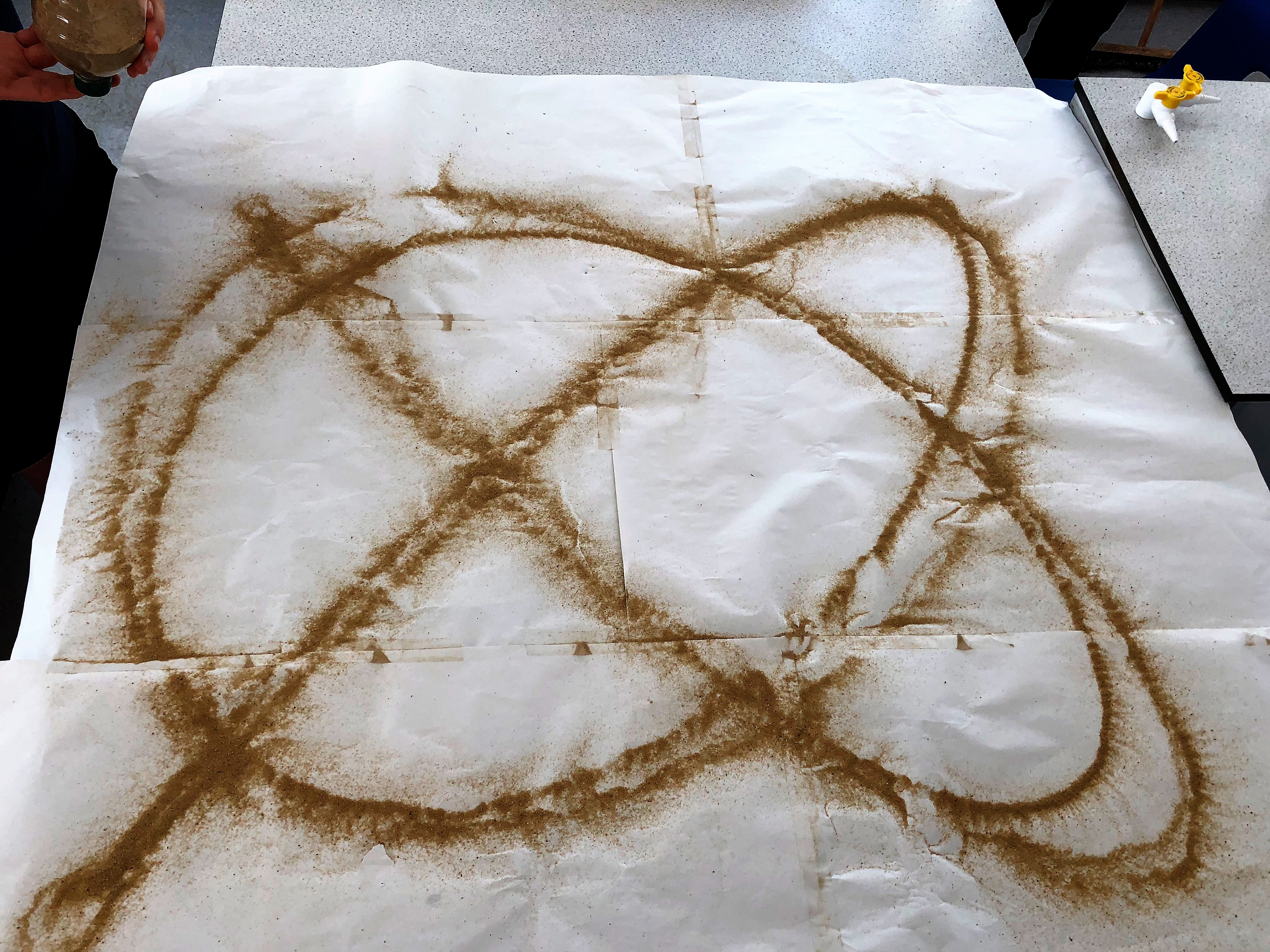
Prior to modern electronic equipment, Lissajous curves could be generated mechanically by means of a harmonograph.

Acoustics

John Tyndall produced Lissajous curves by attaching a small mirror to a tuning fork, and shining a bright light on the mirror. This produced a vertically oscillating bright dot. He then applied a rotating mirror to reflect the dot, producing a spread out curve. He used this technique as an analog oscilloscope to observe and quantify the oscillation patterns of a tuning fork. Later, Helmholtz produced a Lissajous curve as follows. He made an "oscillation microscope" by attaching one lens of a microscope to a tuning fork, so that it oscillated in one direction. He attached a bright dot of paint on a violin string. Then he viewed the dot through the microscope while the string vibrated in the other direction, and saw a Lissajous curve. This is called the "Helmholtz motion".

Practical application

Lissajous curves can also be generated using an oscilloscope (as illustrated). An octopus circuit can be used to demonstrate the waveform images on an oscilloscope. Two phase-shifted sinusoid inputs are applied to the oscilloscope in X-Y mode and the phase relationship between the signals is presented as a Lissajous figure.

In the professional audio world, this method is used for realtime analysis of the phase relationship between the left and right channels of a stereo audio signal. On larger, more sophisticated audio mixing consoles an oscilloscope may be built-in for this purpose.

On an oscilloscope, we suppose x is CH1 and y is CH2, A is the amplitude of CH1 and B is the amplitude of CH2, a is the frequency of CH1 and b is the frequency of CH2, so is the ratio of frequencies of the two channels, and δ is the phase shift of CH1.

A purely mechanical application of a Lissajous curve with , is in the driving mechanism of the Mars Light type of oscillating beam lamps popular with railroads in the mid-1900s. The beam in some versions traces out a lopsided figure-8 pattern on its side.

Application for the case of ''a'' = ''b''

'''Top:''' Output signal as a function of time.<br>'''Middle:''' Input signal as a function of time.<br>'''Bottom:''' Resulting Lissajous curve when output is plotted as a function of the input.<br>In this particular example, because the output is 90 degrees out of phase from that of the input, and the amplitude of the output is the same as the amplitude of the input, the Lissajous curve is a circle, and is rotating counterclockwise.

When the input to a Linear time-invariant (LTI) system is sinusoidal, the output is sinusoidal with the same frequency, but it may have a different amplitude and some phase shift. Using an oscilloscope that can plot one signal against another (as opposed to one signal against time) to plot the output of an LTI system against the input to the LTI system produces an ellipse that is a Lissajous figure for the special case of .

The figure below summarizes how the Lissajous figure changes over different phase shifts for the special case that the output amplitude equals the input amplitude. The phase shifts are representated as negative quantities so that they can be associated with positive (i.e. physical) delay lengths (where the \text{delay length }= -\frac{c}{f}\cdot\frac{\text{phase shift}}{360^\circ}, c is the speed of light, and f is the frequency of the input sinusoidal signal, which is the same as the symbols a and b that define Lissajous curves). The arrows show the direction of rotation of the Lissajous figure.

If the phase shift is 0° or -180°, the resulting Lissajous curve is a line with the slope of the line defined as the ratio of the output amplitude to the input amplitude. If the phase shift is -90° or -270° and the output amplitude equals the input amplitude, the resulting Lissajous curve is a perfect circle.

In engineering

A Lissajous curve is used in experimental tests to determine if a device may be properly categorized as a memristor. It is also used to compare two different electrical signals: a known reference signal and a signal to be tested.

In popular culture

In motion pictures

Lissajous figures were sometimes displayed on oscilloscopes meant to simulate high-tech equipment in science-fiction TV shows and movies in the 1960s and 1970s.
The title sequence by John Whitney for Alfred Hitchcock's 1958 feature film Vertigo is based on Lissajous figures.

Company logos

Lissajous figures are sometimes used in graphic design as logos. Examples of non-trivial (i.e. , , and ) use of Lissajous curves in logos include:

The Australian Broadcasting Corporation (, , )
The Lincoln Laboratory at MIT (, , )
The open air club Else in Berlin (, , )
The University of Electro-Communications, Japan (, , ).
Disney's Movies Anywhere streaming video application uses a stylized version of the curve
Facebook's rebrand into Meta Platforms is also a Lissajous Curve, echoing the shape of a capital letter M (, , ).
Home State Brewing co. Used as their logo and signifying a single moment as well as the passage of time— Ichi-go ichi-e

In modern art

The Dadaist artist Max Ernst painted Lissajous figures directly by swinging a punctured bucket of paint over a canvas.

In music education

Lissajous curves have been used in the past to graphically represent musical intervals through the use of the Harmonograph, a device that consists of pendulums oscillating at different frequency ratios. Because different tuning systems employ different frequency ratios to define intervals, these can be compared using Lissajous curves to observe their differences. Therefore, Lissajous curves have applications in music education by graphically representing differences between intervals and among tuning systems.

Notes

References

Lawrence, J.D.. (1972). "A Cataloge of Special Plane Curves". Dover Publication.
(1989). "Mathematical Models". Tarquin Pub.
Wells, D.. (1991). "The Penguin Dictionary of Curious and Interesting Geometry". Penguin.
Rossing, Thomas. (2007). "A Brief History of Acoustics". Springer, New York, NY.
(September 2011). "Lissajous Figures: An Engineering Tool for Root Cause Analysis of Individual Cases—A Preliminary Concept". The Journal of Extra-corporeal Technology.
"Lissajou Curves".
(24 September 1987). "A long way from Lissajous figures". Reed Business Information.
McCormack, Tom. (9 May 2013). "Did 'Vertigo' Introduce Computer Graphics to Cinema?".
(1998). "The ABC's of Lissajous figures". Australian Broadcasting Corporation.
(2008). "Lincoln Laboratory Logo". [[Massachusetts Institute of Technology]].
(2024). "About Us".
King, M.. (2002). "From Max Ernst to Ernst Mach: epistemology in art and science.".
(1893). "The Harmonograph". Jarrold & Sons Printers.
(2023). "Recurrence in Lissajous Curves and the Visual Representation of Tuning Systems". Foundations of Science.

Info: Wikipedia Source

This article was imported from Wikipedia and is available under the Creative Commons Attribution-ShareAlike 4.0 License. Content has been adapted to SurfDoc format. Original contributors can be found on the article history page.

1815-introductions 1815-in-science plane-curves trigonometry articles-containing-video-clips

Want to explore this topic further?

Ask Mako anything about Lissajous curve — get instant answers, deeper analysis, and related topics.

Research with Mako

Free with your Surf account

Content sourced from Wikipedia, available under CC BY-SA 4.0.

This content may have been generated or modified by AI. CloudSurf Software LLC is not responsible for the accuracy, completeness, or reliability of AI-generated content. Always verify important information from primary sources.

Report