From Surf Wiki (app.surf) — the open knowledge base
68–95–99.7 rule
Shorthand used in statistics
Shorthand used in statistics

In statistics, the 68–95–99.7 rule, also known as the empirical rule or 68–95–99.7 rule for a normal distribution and sometimes abbreviated 3 or is a shorthand used to remember the percentage of values that lie within an interval estimate in a normal distribution: approximately 68%, 95%, and 99.7% of the values lie within one, two, and three standard deviations of the mean, respectively.
In mathematical notation, these facts can be expressed as follows, where Pr() is the probability function, Χ is an observation from a normally distributed random variable, μ (mu) is the mean of the distribution, and σ (sigma) is its standard deviation: \begin{align} \Pr(\mu-1\sigma \le X \le \mu+1\sigma) & \approx 68.27% \ \Pr(\mu-2\sigma \le X \le \mu+2\sigma) & \approx 95.45% \ \Pr(\mu-3\sigma \le X \le \mu+3\sigma) & \approx 99.73% \end{align}
The usefulness of this heuristic depends especially on the question under consideration and the manner in which the data have been collected; most particularly the heuristic depends on the data genuinely being normally distributed: Among the many bell-shaped distributions often seen in real-life data, the normal distribution has notoriously "thin tails" – an unusual concentration of probability near its center. If the datum X is instead governed by one of the many similar-appearing and commonly encountered distributions that have "fatter tails" – with probability more spread-out – the significance would be lower for all three deviations from the mean.
Three-sigma ruleIn the empirical sciences, the so-called three-sigma rule of thumb (or expresses a conventional heuristic that nearly all values are taken to lie within three standard deviations of the mean, and thus it is empirically useful to treat 99.7% probability as near certainty.This use of the phrase "three-sigma rule" became common in the 2000s, e.g. cited in
In the social sciences, a result may be considered statistically significant (clear enough to warrant closer examination) if its confidence level is of the order of a two-sigma effect (95%), while in particle physics, there is a convention of requiring statistical significance of a five-sigma effect (99.99994% confidence) to qualify as a discovery.
A weaker three-sigma rule can be derived from Chebyshev's inequality, stating that even for non-normally distributed variables, at least 88.8% of cases should fall within properly calculated three-sigma intervals. For unimodal distributions, the probability of being within three-sigma is at least 95% by the Vysochanskij–Petunin inequality. There may be certain assumptions for a distribution that force this probability to be at least 98%.See:
Proof
We have that \begin{align}\Pr(\mu -n\sigma \leq X \leq \mu + n\sigma) = \int_{\mu-n\sigma}^{\mu + n\sigma} \frac{1}{\sqrt{2\pi} \sigma} e^{-\frac{1}{2} \left(\frac{x-\mu}{\sigma}\right)^2} dx, \end{align} doing the change of variable in terms of the standard score z = \frac{x - \mu}{\sigma}, we have \begin{align}\frac{1}{\sqrt{2\pi}} \int_{-n}^{n} e^{-\frac{z^2}{2}}dz\end{align}, and this integral is independent of \mu and \sigma. We only need to calculate each integral for the cases n = 1,2,3. \begin{align} \Pr(\mu -1\sigma \leq X \leq \mu + 1\sigma) &= \frac{1}{\sqrt{2\pi}} \int_{-1}^{1} e^{-\frac{z^2}{2}}dz \approx 0.6826894921 \ \Pr(\mu -2\sigma \leq X \leq \mu + 2\sigma) &= \frac{1}{\sqrt{2\pi}}\int_{-2}^{2} e^{-\frac{z^2}{2}}dz \approx 0.9544997361 \ \Pr(\mu -3\sigma \leq X \leq \mu + 3\sigma) &= \frac{1}{\sqrt{2\pi}}\int_{-3}^{3} e^{-\frac{z^2}{2}}dz \approx 0.9973002039. \end{align}
Cumulative distribution function
Main article: Prediction interval#Known mean, known variance
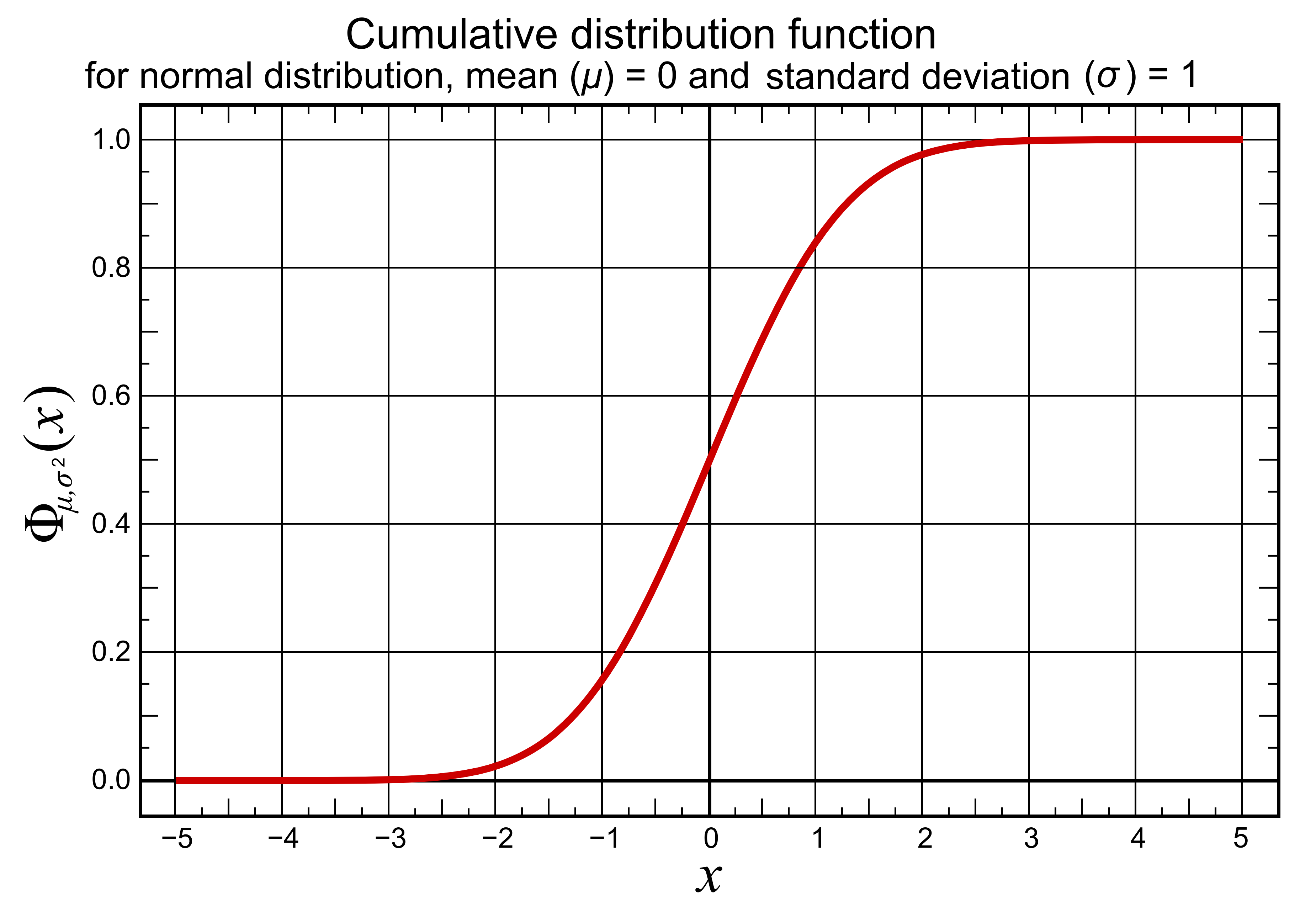
These numerical values "68%, 95%, 99.7%" come from the cumulative distribution function of the normal distribution.
The prediction interval for any standard score z corresponds numerically to .
For example, Φ(2) ≈ 0.9772, or Pr(X ≤ μ + 2σ) ≈ 0.9772, corresponding to a prediction interval of . This is not a symmetrical interval – this is merely the probability that an observation is less than μ + 2σ. To compute the probability that an observation is within two standard deviations of the mean (small differences due to rounding): \Pr(\mu-2\sigma \le X \le \mu+2\sigma) = \Phi(2) - \Phi(-2) \approx 0.9772 - (1 - 0.9772) \approx 0.9545
This is related to confidence interval as used in statistics: \bar{X} \pm 2\frac{\sigma}{\sqrt{n}} is approximately a 95% confidence interval when \bar{X} is the average of a sample of size n.
Normality tests
Main article: Normality test
The "68–95–99.7 rule" is often used to quickly get a rough probability estimate of something, given its standard deviation, if the population is assumed to be normal. It is also used as a simple test for outliers if the population is assumed normal, and as a normality test if the population is potentially not normal.
To pass from a sample to a number of standard deviations, one first computes the deviation, either the error or residual depending on whether one knows the population mean or only estimates it. The next step is standardizing (dividing by the population standard deviation), if the population parameters are known, or studentizing (dividing by an estimate of the standard deviation), if the parameters are unknown and only estimated.
To use as a test for outliers or a normality test, one computes the size of deviations in terms of standard deviations, and compares this to expected frequency. Given a sample set, one can compute the studentized residuals and compare these to the expected frequency: points that fall more than 3 standard deviations from the norm are likely outliers (unless the sample size is significantly large, by which point one expects a sample this extreme), and if there are many points more than 3 standard deviations from the norm, one likely has reason to question the assumed normality of the distribution. This holds ever more strongly for moves of 4 or more standard deviations.
One can compute more precisely, approximating the number of extreme moves of a given magnitude or greater by a Poisson distribution, but simply, if one has multiple 4 standard deviation moves in a sample of size 1,000, one has strong reason to consider these outliers or question the assumed normality of the distribution.
For example, a 6σ event corresponds to a chance of about two parts per billion. For illustration, if events are taken to occur daily, this would correspond to an event expected every 1.4 million years. This gives a simple normality test: if one witnesses a 6σ in daily data and significantly fewer than 1 million years have passed, then a normal distribution most likely does not provide a good model for the magnitude or frequency of large deviations in this respect.
In The Black Swan, Nassim Nicholas Taleb gives the example of risk models according to which the Black Monday crash would correspond to a 36-σ event: according to wolphramalpha.com, a "36-sigma event" corresponds to an expected frequency of the order of 10−215, i.e. beyond astronomically small, perhaps one expected "event" in the history of the universe if events take place every planck time in every planck volume, or something insane like that. this is far beyond the applicability of the "gambler's fallacy", citing gambler's fallacy here would be like calling "gambler's fallacy" if somebody complained about a certain roulette table coming up zero every time during a whole week or so.-- the occurrence of such an event should instantly suggest that the model is flawed, i.e. that the process under consideration is not satisfactorily modeled by a normal distribution. Refined models should then be considered, e.g. by the introduction of stochastic volatility. In such discussions it is important to be aware of the problem of the gambler's fallacy, which states that a single observation of a rare event does not contradict that the event is in fact rare. It is the observation of a plurality of purportedly rare events that increasingly undermines the hypothesis that they are rare, i.e. the validity of the assumed model. A proper modelling of this process of gradual loss of confidence in a hypothesis would involve the designation of prior probability not just to the hypothesis itself but to all possible alternative hypotheses. For this reason, statistical hypothesis testing works not so much by confirming a hypothesis considered to be likely, but by refuting hypotheses considered unlikely.
Table of numerical values
Because of the exponentially decreasing tails of the normal distribution, odds of higher deviations decrease very quickly. From the rules for normally distributed data for a daily event:
| Range | Expected fraction of population | Approx. expected frequency outside range | Approx. frequency outside range for daily event | inside range | outside range |
|---|---|---|---|---|---|
| = 61.71 % | 3 in 5 | Four or five times a week | |||
| *μ* ± *σ* | = 31.73 % | 1 in 3 | Twice or thrice a week | ||
| *μ* ± 1.5 *σ* | = 13.36 % | 2 in 15 | Weekly | ||
| *μ* ± 2 *σ* | = 4.550 % | 1 in 22 | Every three weeks | ||
| *μ* ± 2.5 *σ* | = 1.242 % | 1 in 81 | Quarterly | ||
| *μ* ± 3 *σ* | = 0.270 % = 2.700 ‰ | 1 in 370 | Yearly | ||
| *μ* ± 3.5 *σ* | = 0.04653 % = | 1 in 2149 | Every 6 years | ||
| *μ* ± 4 *σ* | = | 1 in | Every 43 years (twice in a lifetime) | ||
| *μ* ± 4.5 *σ* | = | 1 in | Every 403 years (once in the modern era) | ||
| *μ* ± 5 *σ* | = = | 1 in | Every years (once in recorded history) | ||
| *μ* ± 5.5 *σ* | = | 1 in | Every years (thrice in history of modern humankind) | ||
| *μ* ± 6 *σ* | = | 1 in | Every 1.38 million years (twice in history of humankind) | ||
| *μ* ± 6.5 *σ* | = = | 1 in | Every 34 million years (twice since the extinction of dinosaurs) | ||
| *μ* ± 7 *σ* | = | 1 in | Every 1.07 billion years (four occurrences in history of Earth) | ||
| *μ* ± 7.5 *σ* | = | 1 in | Once every 43 billion years (never in the history of the Universe, twice in the future of the Local Group before its merger) | ||
| *μ* ± 8 *σ* | = | 1 in | Once every 2.2 trillion years (never in the history of the Universe, once during the life of a red dwarf) | ||
| *μ* ± *xσ* | \operatorname{erf}\left(\frac{x}{\sqrt{2}}\right) | 1 - \operatorname{erf}\left(\frac{x}{\sqrt{2}}\right) | 1 in \frac{1}{1 - \operatorname{erf}\left(\frac{x}{\sqrt{2}}\right)} | Every \frac{1}{1 - \operatorname{erf}\left(\frac{x}{\sqrt{2}}\right)} days |
References
References
- (April 9, 2013). "Understanding Advanced Statistical Methods". [[CRC Press]].
- Huber, Franz. (2018). "A Logical Introduction to Probability and Induction". [[Oxford University Press]].
- Lyons, Louis. (7 October 2013). "Discovering the sigificance {{nobr".
- {{Cite OEIS. A178647
- {{cite OEIS. A110894
- {{cite OEIS. A270712
This article was imported from Wikipedia and is available under the Creative Commons Attribution-ShareAlike 4.0 License. Content has been adapted to SurfDoc format. Original contributors can be found on the article history page.
Ask Mako anything about 68–95–99.7 rule — get instant answers, deeper analysis, and related topics.
Research with MakoFree with your Surf account
Create a free account to save articles, ask Mako questions, and organize your research.
Sign up freeThis content may have been generated or modified by AI. CloudSurf Software LLC is not responsible for the accuracy, completeness, or reliability of AI-generated content. Always verify important information from primary sources.
Report