Sinc function

Quality 0.50 · 5 views · Updated 2 months ago

Special mathematical function defined as sin(x)/x

title: "Sinc function" type: doc version: 1 created: 2026-02-28 author: "Wikipedia contributors" status: active scope: public tags: ["signal-processing", "elementary-special-functions"] description: "Special mathematical function defined as sin(x)/x" topic_path: "engineering" source: "https://en.wikipedia.org/wiki/Sinc_function" license: "CC BY-SA 4.0" wikipedia_page_id: 0 wikipedia_revision_id: 0

::summary Special mathematical function defined as sin(x)/x ::

::data[format=table title="Infobox mathematical function"]

Field	Value
name	Sinc
image	Si sinc.svg
imagesize	350px
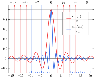
imagealt	Part of the normalized and unnormalized sinc function shown on the same scale
caption	Part of the normalized sinc (blue) and unnormalized sinc function (red) shown on the same scale
general_definition	\operatorname{sinc}x = \begin{cases} \dfrac{ \sin x } x, & x \ne 0 \ 1, & x = 0\end{cases}
fields_of_application	Signal processing, spectroscopy
domain	\mathbb{R}
range	[-0.217234\ldots, 1]
parity	Even
zero	1
plusinf	0
minusinf	0
max	1 at x = 0
min	-0.21723\ldots at x = \pm 4.49341\ldots
root	\pi k, k \in \mathbb{Z}_{\neq 0}
reciprocal	\begin{cases} x \csc x, & x \ne 0 \ 1, & x = 0 \end{cases}
derivative	\operatorname{sinc}'x = \begin{cases} \dfrac{\cos x - \operatorname{sinc} x}{x}, & x \ne 0 \ 0, & x = 0 \end{cases}
antiderivative	\int \operatorname{sinc} x,dx = \operatorname{Si}(x) + C
taylor_series	\operatorname{sinc}x = \sum_{k=0}^\infty \frac{(-1)^k x^{2k
::

| name = Sinc | image = Si sinc.svg | imagesize = 350px | imagealt = Part of the normalized and unnormalized sinc function shown on the same scale | caption = Part of the normalized sinc (blue) and unnormalized sinc function (red) shown on the same scale | general_definition = \operatorname{sinc}x = \begin{cases} \dfrac{ \sin x } x, & x \ne 0 \ 1, & x = 0\end{cases} | fields_of_application = Signal processing, spectroscopy | domain = \mathbb{R} | range = [-0.217234\ldots, 1] | parity = Even | zero = 1 | plusinf = 0 | minusinf = 0 | max = 1 at x = 0 | min = -0.21723\ldots at x = \pm 4.49341\ldots | root = \pi k, k \in \mathbb{Z}{\neq 0} | reciprocal = \begin{cases} x \csc x, & x \ne 0 \ 1, & x = 0 \end{cases} | derivative = \operatorname{sinc}'x = \begin{cases} \dfrac{\cos x - \operatorname{sinc} x}{x}, & x \ne 0 \ 0, & x = 0 \end{cases} | antiderivative = \int \operatorname{sinc} x,dx = \operatorname{Si}(x) + C | taylor_series = \operatorname{sinc}x = \sum{k=0}^\infty \frac{(-1)^k x^{2k}}{(2k + 1)!}

In mathematics, physics and engineering, the sinc function ( ), denoted by sinc(x), is defined as either \operatorname{sinc}(x) = \frac{\sin x}{x}. or \operatorname{sinc}(x) = \frac{\sin \pi x}{\pi x},

the latter of which is sometimes referred to as the normalized sinc function. The only difference between the two definitions is in the scaling of the independent variable (the x axis) by a factor of . In both cases, the value of the function at the removable singularity at zero is understood to be the limit value 1. The sinc function is then analytic everywhere and hence an entire function.

The normalized sinc function is the Fourier transform of the rectangular function with no scaling. It is used in the concept of reconstructing a continuous bandlimited signal from uniformly spaced samples of that signal. The sinc filter is used in signal processing.

The function itself was first mathematically derived in this form by Lord Rayleigh in his expression (Rayleigh's formula) for the zeroth-order spherical Bessel function of the first kind.

The sinc function is also called the cardinal sine function.

Definitions

::figure[src="https://upload.wikimedia.org/wikipedia/commons/4/46/Sinc.wav" caption="The sinc function as audio, at 2000 Hz (±1.5 seconds around zero)"] ::

The sinc function has two forms, normalized and unnormalized.

In mathematics, the historical unnormalized sinc function is defined for x ≠ 0 by \operatorname{sinc}(x) = \frac{\sin x}{x}.

Alternatively, the unnormalized sinc function is often called the sampling function, indicated as Sa(x).

In digital signal processing and information theory, the normalized sinc function is commonly defined for x ≠ 0 by \operatorname{sinc}(x) = \frac{\sin(\pi x)}{\pi x}.

In either case, the value at is defined to be the limiting value \operatorname{sinc}(0) := \lim_{x \to 0}\frac{\sin(a x)}{a x} = 1 for all real a ≠ 0 (the limit can be proven using the squeeze theorem).

The normalization causes the definite integral of the function over the real numbers to equal 1 (whereas the same integral of the unnormalized sinc function has a value of ). As a further useful property, the zeros of the normalized sinc function are the nonzero integer values of x.

Etymology

The function has also been called the cardinal sine or sine cardinal function. The term "sinc" is a contraction of the function's full Latin name, the sinus cardinalis It is also used in Woodward's 1953 book Probability and Information Theory, with Applications to Radar.

Properties

::figure[src="https://upload.wikimedia.org/wikipedia/commons/5/5f/Si_cos.svg" caption="The local maxima and minima (small white dots) of the unnormalized, red sinc function correspond to its intersections with the blue [[cosine function]]."] ::

The zero crossings of the unnormalized sinc are at non-zero integer multiples of , while zero crossings of the normalized sinc occur at non-zero integers.

The local maxima and minima of the unnormalized sinc correspond to its intersections with the cosine function. That is, for all points ξ where the derivative of is zero and thus a local extremum is reached. This follows from the derivative of the sinc function: \frac{d}{dx}\operatorname{sinc}(x) = \begin{cases} \dfrac{\cos(x) - \operatorname{sinc}(x)}{x}, & x \ne 0 \0, & x = 0\end{cases}.

The first few terms of the infinite series for the x coordinate of the n-th extremum with positive x coordinate are x_n = q - q^{-1} - \frac{2}{3} q^{-3} - \frac{13}{15} q^{-5} - \frac{146}{105} q^{-7} - \cdots, where q = \left(n + \frac{1}{2}\right) \pi, and where odd n lead to a local minimum, and even n to a local maximum. Because of symmetry around the y axis, there exist extrema with x coordinates −xn. In addition, there is an absolute maximum at .

The normalized sinc function has a simple representation as the infinite product: \frac{\sin(\pi x)}{\pi x} = \prod_{n=1}^\infty \left(1 - \frac{x^2}{n^2}\right) ::figure[src="https://upload.wikimedia.org/wikipedia/commons/0/08/The_cardinal_sine_function_sinc(z)plotted_in_the_complex_plane_from-2-2i_to_2+2i.svg" caption="The cardinal sine function sinc(z) plotted in the complex plane from -2-2i to 2+2i" alt="The cardinal sine function sinc(z) plotted in the complex plane from -2-2i to 2+2i"] ::

and is related to the gamma function Γ(x) through Euler's reflection formula: \frac{\sin(\pi x)}{\pi x} = \frac{1}{\Gamma(1 + x)\Gamma(1 - x)}.

Euler discovered that \frac{\sin(x)}{x} = \prod_{n=1}^\infty \cos\left(\frac{x}{2^n}\right), and because of the product-to-sum identity ::figure[src="https://upload.wikimedia.org/wikipedia/commons/d/d5/Sinc_cplot.svg" caption="''z''}}}}"] ::

\prod_{n=1}^k \cos\left(\frac{x}{2^n}\right) = \frac{1}{2^{k-1}} \sum_{n=1}^{2^{k-1}} \cos\left(\frac{n - 1/2}{2^{k-1}} x \right),\quad \forall k \ge 1, Euler's product can be recast as a sum \frac{\sin(x)}{x} = \lim_{N\to\infty} \frac{1}{N} \sum_{n=1}^N \cos\left(\frac{n - 1/2}{N} x\right).

The continuous Fourier transform of the normalized sinc (to ordinary frequency) is rect(f): \int_{-\infty}^\infty \operatorname{sinc}(t) , e^{-i 2 \pi f t},dt = \operatorname{rect}(f), where the rectangular function is 1 for argument between − and , and zero otherwise. This corresponds to the fact that the sinc filter is the ideal (brick-wall, meaning rectangular frequency response) low-pass filter.

This Fourier integral, including the special case \int_{-\infty}^\infty \frac{\sin(\pi x)}{\pi x} , dx = \operatorname{rect}(0) = 1 is an improper integral (see Dirichlet integral) and not a convergent Lebesgue integral, as \int_{-\infty}^\infty \left|\frac{\sin(\pi x)}{\pi x} \right| ,dx = +\infty.

The normalized sinc function has properties that make it ideal in relationship to interpolation of sampled bandlimited functions:

It is an interpolating function, i.e., , and for nonzero integer k.
The functions (k integer) form an orthonormal basis for bandlimited functions in the function space L2(R), with highest angular frequency (that is, highest cycle frequency ).

Other properties of the two sinc functions include:

The unnormalized sinc is the zeroth-order spherical Bessel function of the first kind, j0(x). The normalized sinc is j0(πx).
where Si(x) is the sine integral, \int_0^x \frac{\sin(\theta)}{\theta},d\theta = \operatorname{Si}(x).
λ sinc(λx) (not normalized) is one of two linearly independent solutions to the linear ordinary differential equation x \frac{d^2 y}{d x^2} + 2 \frac{d y}{d x} + \lambda^2 x y = 0. The other is , which is not bounded at , unlike its sinc function counterpart.
Using normalized sinc, \int_{-\infty}^\infty \frac{\sin^2(\theta)}{\theta^2},d\theta = \pi \quad \Rightarrow \quad \int_{-\infty}^\infty \operatorname{sinc}^2(x),dx = 1,
\int_{-\infty}^\infty \frac{\sin(\theta)}{\theta},d\theta = \int_{-\infty}^\infty \left( \frac{\sin(\theta)}{\theta} \right)^2 ,d\theta = \pi.
\int_{-\infty}^\infty \frac{\sin^3(\theta)}{\theta^3},d\theta = \frac{3\pi}{4}.
\int_{-\infty}^\infty \frac{\sin^4(\theta)}{\theta^4},d\theta = \frac{2\pi}{3}.
The following improper integral involves the (not normalized) sinc function: \int_0^\infty \frac{dx}{x^n + 1} = 1 + 2\sum_{k=1}^\infty \frac{(-1)^{k+1}}{(kn)^2 - 1} = \frac{1}{\operatorname{sinc}(\frac{\pi}{n})}.

Relationship to the Dirac delta distribution

The normalized sinc function can be used as a nascent delta function, meaning that the following weak limit holds:

\lim_{a \to 0} \frac{\sin\left(\frac{\pi x}{a}\right)}{\pi x} = \lim_{a \to 0}\frac{1}{a} \operatorname{sinc}\left(\frac{x}{a}\right) = \delta(x).

This is not an ordinary limit, since the left side does not converge. Rather, it means that

\lim_{a \to 0}\int_{-\infty}^\infty \frac{1}{a} \operatorname{sinc}\left(\frac{x}{a}\right) \varphi(x) ,dx = \varphi(0)

for every Schwartz function, as can be seen from the Fourier inversion theorem. In the above expression, as a → 0, the number of oscillations per unit length of the sinc function approaches infinity. Nevertheless, the expression always oscillates inside an envelope of ±, regardless of the value of a.

This complicates the informal picture of δ(x) as being zero for all x except at the point , and illustrates the problem of thinking of the delta function as a function rather than as a distribution. A similar situation is found in the Gibbs phenomenon.

We can also make an immediate connection with the standard Dirac representation of \delta(x) by writing b=1/a and

\lim_{b \to \infty} \frac{\sin\left(b\pi x\right)}{\pi x} = \lim_{b \to \infty} \frac{1}{2\pi} \int_{-b\pi}^{b\pi} e^{ik x}dk= \frac{1}{2\pi} \int_{-\infty}^\infty e^{i k x} dk=\delta(x),

which makes clear the recovery of the delta as an infinite bandwidth limit of the integral.

Summation

All sums in this section refer to the unnormalized sinc function.

The sum of sinc(n) over integer n from 1 to ∞ equals :

\sum_{n=1}^\infty \operatorname{sinc}(n) = \operatorname{sinc}(1) + \operatorname{sinc}(2) + \operatorname{sinc}(3) + \operatorname{sinc}(4) +\cdots = \frac{\pi - 1}{2}.

The sum of the squares also equals :

\sum_{n=1}^\infty \operatorname{sinc}^2(n) = \operatorname{sinc}^2(1) + \operatorname{sinc}^2(2) + \operatorname{sinc}^2(3) + \operatorname{sinc}^2(4) + \cdots = \frac{\pi - 1}{2}.

When the signs of the addends alternate and begin with +, the sum equals : \sum_{n=1}^\infty (-1)^{n+1},\operatorname{sinc}(n) = \operatorname{sinc}(1) - \operatorname{sinc}(2) + \operatorname{sinc}(3) - \operatorname{sinc}(4) + \cdots = \frac{1}{2}.

The alternating sums of the squares and cubes also equal : \sum_{n=1}^\infty (-1)^{n+1},\operatorname{sinc}^2(n) = \operatorname{sinc}^2(1) - \operatorname{sinc}^2(2) + \operatorname{sinc}^2(3) - \operatorname{sinc}^2(4) + \cdots = \frac{1}{2},

\sum_{n=1}^\infty (-1)^{n+1},\operatorname{sinc}^3(n) = \operatorname{sinc}^3(1) - \operatorname{sinc}^3(2) + \operatorname{sinc}^3(3) - \operatorname{sinc}^3(4) + \cdots = \frac{1}{2}.

Series expansion

The Taylor series of the unnormalized sinc function can be obtained from that of the sine (which also yields its value of 1 at ): \frac{\sin x}{x} = \sum_{n=0}^\infty \frac{(-1)^n x^{2n}}{(2n+1)!} = 1 - \frac{x^2}{3!} + \frac{x^4}{5!} - \frac{x^6}{7!} + \cdots

The series converges for all x. The normalized version follows easily: \frac{\sin \pi x}{\pi x} = 1 - \frac{\pi^2x^2}{3!} + \frac{\pi^4x^4}{5!} - \frac{\pi^6x^6}{7!} + \cdots

Euler famously compared this series to the expansion of the infinite product form to solve the Basel problem.

Higher dimensions

The product of 1-D sinc functions readily provides a multivariate sinc function for the square Cartesian grid (lattice): , whose Fourier transform is the indicator function of a square in the frequency space (i.e., the brick wall defined in 2-D space). The sinc function for a non-Cartesian lattice (e.g., hexagonal lattice) is a function whose Fourier transform is the indicator function of the Brillouin zone of that lattice. For example, the sinc function for the hexagonal lattice is a function whose Fourier transform is the indicator function of the unit hexagon in the frequency space. For a non-Cartesian lattice this function can not be obtained by a simple tensor product. However, the explicit formula for the sinc function for the hexagonal, body-centered cubic, face-centered cubic and other higher-dimensional lattices can be explicitly derived using the geometric properties of Brillouin zones and their connection to zonotopes.

For example, a hexagonal lattice can be generated by the (integer) linear span of the vectors \mathbf{u}_1 = \begin{bmatrix} \frac{1}{2} \ \frac{\sqrt{3}}{2} \end{bmatrix} \quad \text{and} \quad \mathbf{u}_2 = \begin{bmatrix} \frac{1}{2} \ -\frac{\sqrt{3}}{2} \end{bmatrix}.

Denoting \boldsymbol{\xi}_1 = \tfrac{2}{3} \mathbf{u}_1, \quad \boldsymbol{\xi}_2 = \tfrac{2}{3} \mathbf{u}_2, \quad \boldsymbol{\xi}_3 = -\tfrac{2}{3} (\mathbf{u}_1 + \mathbf{u}2), \quad \mathbf{x} = \begin{bmatrix} x \ y\end{bmatrix}, one can derive the sinc function for this hexagonal lattice as \begin{align} \operatorname{sinc}\text{H}(\mathbf{x}) = \tfrac{1}{3} \big( & \cos\left(\pi\boldsymbol{\xi}_1\cdot\mathbf{x}\right) \operatorname{sinc}\left(\boldsymbol{\xi}_2\cdot\mathbf{x}\right) \operatorname{sinc}\left(\boldsymbol{\xi}_3\cdot\mathbf{x}\right) \ & {} + \cos\left(\pi\boldsymbol{\xi}_2\cdot\mathbf{x}\right) \operatorname{sinc}\left(\boldsymbol{\xi}_3\cdot\mathbf{x}\right) \operatorname{sinc}\left(\boldsymbol{\xi}_1\cdot\mathbf{x}\right) \ & {} + \cos\left(\pi\boldsymbol{\xi}_3\cdot\mathbf{x}\right) \operatorname{sinc}\left(\boldsymbol{\xi}_1\cdot\mathbf{x}\right) \operatorname{sinc}\left(\boldsymbol{\xi}_2\cdot\mathbf{x}\right) \big). \end{align}

This construction can be used to design Lanczos window for general multidimensional lattices.

Sinhc

Some authors, by analogy, define the hyperbolic sine cardinal function.

:\mathrm{sinhc}(x) = \begin{cases} {\displaystyle \frac{\sinh(x)}{x},} & \text{if }x \ne 0 \ {\displaystyle 1,} & \text{if }x = 0 \end{cases}

References

"Numerical methods".
(2008). "Communication Systems, 2E". Tata McGraw-Hill Education.
Weisstein, Eric W.. "Sinc Function".
Merca, Mircea. (2016-03-01). "The cardinal sine function and the Chebyshev–Stirling numbers". Journal of Number Theory.
(March 1952). "Information theory and inverse probability in telecommunication". Proceedings of the IEE - Part III: Radio and Communication Engineering.
Poynton, Charles A.. (2003). "Digital video and HDTV". Morgan Kaufmann Publishers.
Woodward, Phillip M.. (1953). "Probability and information theory, with applications to radar". Pergamon Press.
Euler, Leonhard. (1735). "On the sums of series of reciprocals".
(2015). "Sampling by incomplete cosine expansion of the sinc function: Application to the Voigt/complex error function". Appl. Math. Comput..
(June–July 1980). "Advanced Problem 6241". [[Mathematical Association of America]].
(December 2008). "Surprising Sinc Sums and Integrals". American Mathematical Monthly.
Baillie, Robert. (2008). "Fun with Fourier series".
(June 2012). "A Geometric Construction of Multivariate Sinc Functions". IEEE Transactions on Image Processing.
Ainslie, Michael. (2010). "Principles of Sonar Performance Modelling". Springer.
Günter, Peter. (2012). "Nonlinear Optical Effects and Materials". Springer.
Schächter, Levi. (2013). "Beam-Wave Interaction in Periodic and Quasi-Periodic Structures". Springer.

::callout[type=info title="Wikipedia Source"] This article was imported from Wikipedia and is available under the Creative Commons Attribution-ShareAlike 4.0 License. Content has been adapted to SurfDoc format. Original contributors can be found on the article history page. ::